Standard Deviation: What It Measures and When the Mean Misleads
Two datasets with the same mean can behave nothing alike — how standard deviation is built step by step, and when to divide by n versus n−1
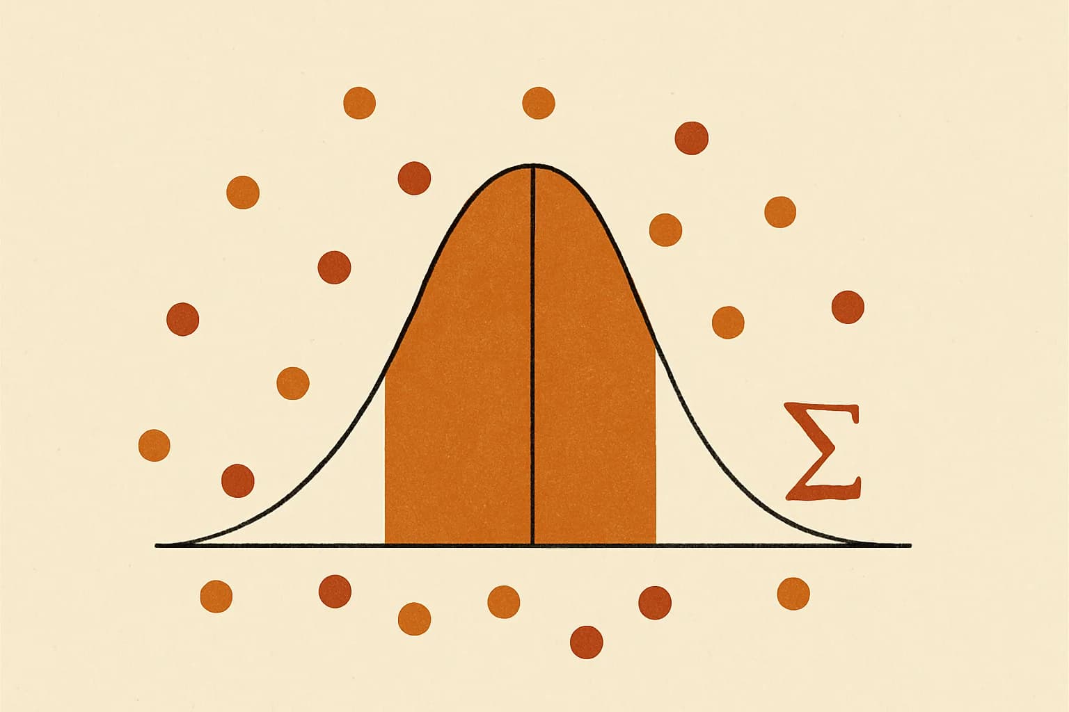
Two commute routes both average 30 minutes. Route A, logged over five days: 28, 29, 30, 31, 32 minutes. Route B, same week: 10, 20, 30, 40, 50. Each log sums to 150, and 150 ÷ 5 = 30, so their means are identical — yet Route A is a commute you can set a watch by, while Route B decides at random whether you make the 9:00 meeting. The mean cannot tell these routes apart, because it answers only one question: where is the middle? Standard deviation answers the question it skips: how far does a typical value sit from that middle?
That is the whole concept. Standard deviation is the typical distance between an observation and the mean, expressed in the same units as the data — minutes here, dollars or kilograms elsewhere. Route A's standard deviation comes out near 1.4 minutes: an ordinary day lands within a minute or two of 30. Route B's is about 14.1 minutes: an "ordinary day" barely exists. Everything else in this post — the n versus n − 1 argument, z-scores, the 68–95–99.7 rule — is machinery built on that one idea.
Watching the number get made
Four steps, worked on Route A:
- Find the mean. 28 + 29 + 30 + 31 + 32 = 150, and 150 ÷ 5 = 30.
- Measure each deviation. Subtracting 30 from each value gives −2, −1, 0, +1, +2. Notice they cancel to zero — deviations from a mean always do, which is why simply averaging them tells you nothing.
- Square and add. Squaring kills the minus signs and weights far-flung values more heavily: 4 + 1 + 0 + 1 + 4 = 10, the sum of squared deviations.
- Divide, then un-square. 10 ÷ 5 = 2 is the variance — spread measured in squared units, minutes². The square root brings it back to minutes: √2 ≈ 1.414.
σ = √[ Σ(xᵢ − x̄)² ⁄ n ]
Run Route B through the same mill: deviations −20, −10, 0, +10, +20 square to 400 + 100 + 0 + 100 + 400 = 1,000, then 1,000 ÷ 5 = 200 and √200 ≈ 14.142 minutes. Same mean, ten times the spread, visible in a single number. The standard deviation calculator performs all four steps on any pasted list and reports both divisor variants alongside the mean, the variances and the count.
Dividing by n − 1: the honest version
Step 4 hid a decision. Dividing by n = 5 gave the population standard deviation, σ — correct if those five days are everything you care about, a closed book. But if the five days are a sample standing in for a longer commuting life you want to generalise about, the convention changes: divide by n − 1 instead, giving the sample standard deviation, s = √[ Σ(xᵢ − x̄)² ⁄ (n − 1) ]. For Route A that means 10 ÷ 4 = 2.5 and √2.5 ≈ 1.581 minutes — and since 1.581 ÷ 1.414 ≈ 1.118, the two answers sit about 12% apart on identical data.
Here is the reason, without hand-waving. The mean you subtracted in step 2 was computed from the same five numbers you then measured against it — and the mean is, by construction, the exact point that makes the sum of squared deviations as small as it can possibly be. Your true long-run average commute is almost certainly not exactly 30.000 minutes, and deviations measured from that unknown true mean would come out somewhat larger. A sample's sum of squares is therefore a systematic underestimate, and dividing by n − 1 rather than n inflates it back by, on average, precisely the right amount. This is Bessel's correction, from Friedrich Bessel's 1838 paper. The degrees-of-freedom framing says the same thing another way: because the five deviations must cancel to zero, only four of them are free to vary — the fifth is forced.
Two honest footnotes that most explainers skip. First, the correction unbiases the variance s², not the standard deviation itself; taking the square root afterwards reintroduces a small bias that statisticians simply live with. Second, the entire controversy is a small-sample affair:
| n | s² ÷ σ² = n ⁄ (n − 1) | Variance inflation |
|---|---|---|
| 2 | 2 ÷ 1 = 2.000 | 100% |
| 5 | 5 ÷ 4 = 1.250 | 25% |
| 10 | 10 ÷ 9 ≈ 1.111 | about 11% |
| 100 | 100 ÷ 99 ≈ 1.010 | about 1% |
| 1,000 | 1,000 ÷ 999 ≈ 1.001 | about 0.1% |
By a few hundred observations the two formulas agree to several decimal places and the argument dissolves.
Choosing between them is a question about your data, not your taste:
| Your dataset is… | Divide by | Symbol | Typical case |
|---|---|---|---|
| every member of the group in question | n | σ | every game of a finished season; every employee on one payroll |
| a sample drawn from a larger whole | n − 1 | s | 30 bulbs from a production run of 100,000; ten scores from a class of forty |
Software mirrors the split, with traps. Excel's STDEV.S uses n − 1 while STDEV.P uses n; R's sd() defaults to the sample version; NumPy's np.std defaults to the population version unless you pass ddof=1 — a mismatch that silently changes answers on exactly the small datasets where the gap is biggest.
What one standard deviation buys you
For roughly bell-shaped data, the mean and standard deviation together become a map. The empirical rule — better known as the 68–95–99.7 rule — says about 68% of values fall within one standard deviation of the mean, about 95% within two, and about 99.7% within three (more precisely 68.27%, 95.45% and 99.73%).
A z-score turns that map into a ranking for a single value: z = (x − mean) ÷ σ. IQ tests are normed to a mean of 100 with σ = 15, so a score of 130 works out as 130 − 100 = 30, then 30 ÷ 15 = 2 — exactly two standard deviations up, which the normal curve places at the 97.72nd percentile, the top 2.28% of the population. The z-score calculator reads the percentile off the normal distribution for you, along with a two-sided p-value. One refinement worth carrying: the exact cutoff enclosing 95% of the curve is z = 1.96, not the mnemonic 2.
The fine print matters, though. Those percentages belong to approximately normal data only. For a skewed distribution the sole universal guarantee is Chebyshev's inequality: at least 75% of any dataset lies within two standard deviations of its mean and at least 89% within three, whatever the shape.
Why the squared version won't retire
Variance looks like standard deviation's rough draft — Route A's 2 minutes² against Route B's 200 minutes² reads awkwardly, and squaring exaggerates the contrast (200 ÷ 2 = 100, a hundredfold gap, where the standard deviations differ only tenfold). But variance owns the property its square root gave up: for independent quantities, variances add — Var(X + Y) = Var(X) + Var(Y). That additivity is the engine inside ANOVA's between-group and within-group decomposition and inside the R² printed on every regression summary, which is why the variance calculator exists as its own tool with an explicit sample/population selector rather than as a footnote to this one.
Reading an average that arrives alone
Three habits guard against a naked mean. Ask for the spread — Routes A and B are indistinguishable without it. Ask which divisor was used whenever n is small — at n = 5 that silent choice moved our answer by roughly 12%. And treat a standard deviation of exactly zero with suspicion: it means every recorded value was identical, which in real measured data usually points to a truncated export or a defaulted field rather than a perfectly steady process.
Every figure in this post reduces to subtraction, squaring, one division and a square root — arithmetic compact enough to audit on an index card, which is worth doing once by hand before trusting any tool with it. When a dataset stops fitting on the card, the three calculators above live alongside the rest of Quanta. And if some step still reads as hand-waving — the degrees-of-freedom argument earns that suspicion more than the others — say so: an explanation of n − 1 only counts as finished once it has survived a skeptical reader.
Sources
- NIST/SEMATECH e-Handbook of Statistical Methods §1.3.5.6 — measures of scale, including the n−1 sample variance
- NIST/SEMATECH e-Handbook §1.3.6.6.1 — the normal distribution
- OpenStax — Introductory Statistics (variance and standard deviation)
- Bessel (1838) — the original treatment of observation errors, Astronomische Nachrichten